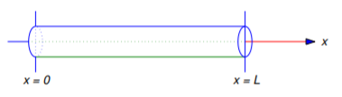
偏微分方程式の勉強を始めるにあたり、まず、長さ(L)が一様で、一端を原点とし、他端を(x=L)とする棒(図)に熱が流れる問題から始めることにしましょう。
棒は端点を除いて完全に絶縁されており、温度は各断面において一定であり、従ってそれは、 \(x\) と \(t\) にのみ依存すると仮定します。 また、棒の熱的特性は \(x), \(t) に依存しないと仮定する。 このとき、原点から単位距離の点(x)における時間(t)の温度(u = u(x, t)\) は偏微分方程式
(ここで、(a)は熱的性質により決まる正の定数) を満たすことができる。 これは熱の方程式である。
To determine \(u}) must specify the temperature at every point in the bar when \(t=0}, say
これを初期条件と呼びます。 また、棒の両端において、すべての \(t>0
) に対して、 \(u} が満たすべき境界条件を指定しなければならない。 この問題を初期境界値問題と呼ぶことにする。
まず境界条件として \(u(0,t)=u(L,t)=0
を指定して、初期境界値問題を
この問題の解法は変数分離と呼ぶ(常微分方程式を解くために第2・2章で使う変数分離の方法と混同しないでね)。 まず、同一ゼロでなく、all \((x,t)\) for allを満たす
形式の関数を探すことから始める。 Since
Think(v_t=a^2v_{xx}}) if and only if
which we rewrite as
Since the left is independent of \(x) while the one is independent of \(tải), この式は、両辺が同じ定数(ここでは分離定数と呼びます)に等しい場合にのみ、すべての \((x,t)\) に対して成り立つことができ、それを \(-lambda**) と表記します。 したがって、
This is equivalent to
and
Since \(v(0.),t)=X(0)T(t)=0) and \(v(L,t)=X(L)T(t)=0) and we don’t want to be identically zero, \(X(0)=0) and \(X(L)=0). 従って、境界値問題
の固有値であることが必要であり、 \(X)-eigenfunction であることが必要である。 定理11.1.2より、方程式の固有値は \(\lambda_n=n^2pi^2/L^2), associated eigenfunction
Substituting \ref{eq:12.1.2} となり、解
が得られる。ここで、
Since
Thomas (v_n} satisfilling Equation \ref{eq:12.1.1} with \(f(x)=TEINSIN NÄMI x/LTEIN). もっと一般的に言うと、 \(u_m**) が Equation \{eq:12.1.1} with
を満たすとすると、次の定義が動機付けられます。
Theorem \(\PageIndex{1})
The formal solution of the initial-…境界値問題
is
where
is Fourier sine series of \(fante) on (\); that is,
\
We use the term “formal solution” in this definition because it is not general true that the infinite series in Equation \ref{eq:12.1.5}の無限級数が初期境界値問題Equation \ref{eq:12.1.4} のすべての要件を満たすとき、Equation \ref{eq:12.1.4} の実際の解であると言うので、この定義を使用します。1.4}.
Because the negative exponentials in Equation \ref{eq:12.1.5}, \(u) converges for all \((x,t)\ with \(t>0}) (Exercise 12.1.54). 式{eq:12.1.5}の各項は熱方程式を満たし、式{eq:12.1.5}の境界条件を満たすので、式{eq:12.1.5}の境界条件は満たされます。4}の熱方程式と境界条件を満たすので、Equation \ref{eq:12.1.5} の系列を1項ずつ微分して、 \(t>0} の場合は \(u_t}) と \(u_{xx}) が得られれば、これらの性質も満たします。 しかし、無限級数を一項ずつ微分することは必ずしも正統ではない。 次の定理は無限級数のterm by termの微分が正統であるための有用な十分条件を与える。 証明は省略する。
Theorem \(\PageIndex{2})
A convergent infinite series
can be differentiated by term term by term on a closed interval ╱╱╱╱╱╱で導関数が1つになる。\(w_n’\) is continuous on \(\) and
where \(M_1,\) \(M_2,\) …, \(M_n,\) …, is constants that that series \(sum_{n=1}^infty M_n}) converges.
Theorem ⒶをⒶとⒷで2回適用すると、Ⓐを項ごとに微分すると、(t>0)のとき、(u_{xx})、(u_t})が得られることがわかります(演習12.1.54). 従って、(t>0)の場合、(u_t)は熱方程式と境界条件(式)を満たします。 従って、”u(x,0)=S(x)week” for \(0le xxxle Lxx)から、”u(x) “はEquation \ref{eq:12.1.4} if and only if \(S(x)=f(x)une) for 0´ xxxle Lxx)の実解であると言えるのです。 定理11.3.2より、これは \(f) is continuous and piecewise smooth on \(L), and \(f(0)=f(L)=0) のときに真となります。
この章ではいくつかの種類の問題に対する形式解を定義しています。
例題 \(\PageIndex{1})
Solve Equation \ref{eq:12.1.4} with \(f(x)=x(x^2-3Lx+2L^2)Раааааа).
Solution
From Example \ is
Therefore
Three
If both ends of bar is insulated so that can no heat pass through, then the boundary conditions are
We leave you (Exercise 12. ) the pastary conditions are We were relatively to you to the other than the pastary conditions is The other of bar is
Three than two sides of the pasties are Three than two sides of the bar is Three than two sides of the pasties are
Theorem \(\PageIndex{3})
The formal solution of the initial-boundary value problem
is
where
is the Fourier cosine series of \(fenta) on \(.), and the Fourier cosine series of \(fàn) on the \;12.1.6}を㊙(f(x)=x㊙)で解きます。
Solution
例題11.3.1より, \(f) on \(f) のFourier cosine seriesは
Therefore
There is you (Exercise 12.)
We leave it to you (Exercise 12.).1.2)で変数分離法と定理11.1.4を使って、次の定義の動機付けを行うことにしよう。
Theorem \(\PageIndex{4})
The formal solution of the initial-boundary value problem
is
where
is the mixed Fourier sine series of \(fenta) on \(.NET);12.1.7} with \(f(x)=x}.
Solution
From Example 11.3.4より、(f)の混合フーリエサイン系列は
Therefore
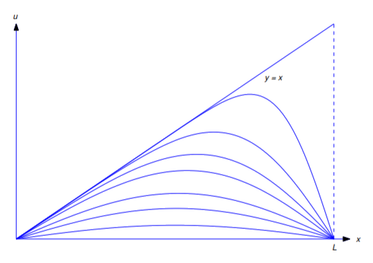
Figure \(PageIndex{2}) is a graph plotted with \(x} for various values of tenta.)。 線分(y=x)は(t=0)に対応します。 他の曲線は、正の値を持つ閾値に対応しています。 ⑭(t)が増加すると、グラフは線分⑯(u=0)に近づく。
We leave you to (Exercise 12.1.3) use the method of separation of variables and Theorem 11.1.5 to motivate the next definition.
Theorem \(\PageIndex{5})
The formal solution of the initial->
Theorem 11.1.5.5の定義に従う。ここで、
は、Mixed Fourier cosine series of \(fenta) on (\) である。 that is,
Example \(\PageIndex{4})
Solve Equation \{eq.weeks}。12.1.8}をⒶ(f(x)=x-Lalink).で解く
From Example 11.3.1.3より, Ⓐの混合フーリエ余弦級数は
Therefore
Threshold
Using Technology
数値実験により初期境界値問題の解についての理解を深めることができます。 具体的には、式≪ref{eq:12.1.4}≫の形式解
は、Fourier sine series of \(f) on \(\) である。 For several fixed values of \(t) (including \(t=0jee)), graph \(u_m(x,t)\) versus \(t). In cases may be useful to graph the curves corresponding to various values of \(tenta) on the same axes and other cases you want to graph the various curves successively (for increasing values of \(tenta)), and create a primitive motion picture on your monitor.場合によっては、同じ軸の上に、様々な値に対応する曲線をグラフ化することが有用である。 また、この実験を何度か繰り返して、”plimitive motion picture “を作成し、 \(tenta) の値が小さいときと大きいときで、”plimitive motion picture “の結果がどのように変化するかを比較することができます。 ただし、この場合の「小さい」「大きい」の意味は、定数 \(a^2คi), \(L^2คi) に依存することに留意してください。 これを扱うには、式
where
を書き換えて、selected values of \(u_matta) versus \(x) graph for selected values of \(\tau) とすればよいでしょう。
これらのコメントは、Theorems Ⓐ(\PageIndex{3}) -Ⓑ(\PageIndex{5}) で考慮した状況にも適用できますが、Equation \ref{eq:12}は例外です。1.13}は、Theorems ⑅(\PageIndex{4}) and ⑅(\PageIndex{5}).
に置き換える必要があります。